Interpretable Neural Networks

Interpreting black box models is a significant challenge in machine learning, and can significantly reduce barriers to adoption of the technology.

In a previous post, I discussed interpreting complex machine learning models using shap values. To summarize, for a particular feature, the prediction of a model for a specific data point is compared when it can see the feature, and when it can’t — the magnitude of this difference tells us how important that feature is to the model’s prediction.

In the example below, we have built a model to predict whether someone wants ice cream, and it consists of three features: whether they like cold foods, the season they are in right now and whether they like sweet foods. Shap values allow us to explain the output of the model for individual data points — in this case, for Bob:

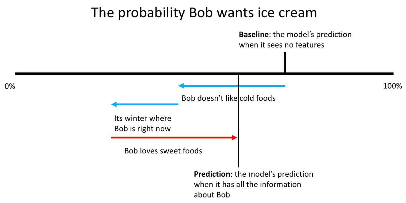
There are two things to note from this ice cream model: firstly, the effect of the features is being compared to a baseline of what the model would predict when it can’t see the features. Secondly, the sum of the feature importances (the red and blue arrows) is the difference between this baseline and the model’s actual prediction for Bob.

Unfortunately, while certain machine learning algorithms (such as XGBoost) can handle null feature values (i.e. not seeing a feature), neural networks can’t, so a slightly different approach will be needed to interpret them. The most common approach so far has been to consider the gradients of the inputs with respect to the predictions.

In this post, I will cover the intuition behind using these gradients, as well as two specific techniques that have come out of this: Integrated Gradients and DeepLift.

Using gradients to interpret neural networks

Possibly the most intepretable model — and therefore the one we will use as inspiration — is a regression. In a regression, each feature \( x \) is assigned some weight, \( w \), which directly tells me that feature’s importance to the model.

Specifically, for the \(i^{th} \) feature of a specific data point, the feature’s contribution to the model output is \( w_{i} \times x_{i} \).

What does this weight \( w \) represent? Well, since a regression is

\[ Y = (w_{1}x_{1} + … + w_{i}x_{i} + … + w_{n}x_{n}) + b \]

Then

\[ w_{i} = \frac{\partial Y}{\partial x_{i}} \]

In other words, the weight assigned to the ith feature tells us the gradient of that feature with respect to the model’s prediction: how the model’s prediction changes as the feature changes.

Conveniently, this gradient is easy to calculate for neural networks. So, in the same way that for a regression, a feature’s contribution is \( (w_{i}x_{i} = \frac{\partial Y}{\partial x_{i}} x_{i}) \), perhaps the gradient can be used to explain the output of a neural network.

There are two issues we run into when trying to use this approach:

Firstly, feature importances are relative. For gradient boosted decision trees, a feature’s shap value tells me how a feature changed the prediction of the model relative to the model not seeing that feature. Since neural networks can’t handle null input features, we’ll need to redefine a feature’s impact relative to something else.

To overcome this, we’ll define a new baseline: what am I comparing my input against? One example is for the MNIST digits dataset. Since all the digits are white, against a black background, perhaps a reasonable background would be a fully black image, since this represents no information about the digits:

Choosing a background for other datasets is much less trivial — for instance, what should the background be for the ImageNet dataset? We’ll discuss a solution for this later, but for now let’s assume that we can find a baseline for each dataset.

The second issue is that using the gradient of the output with respect to the input works well for a linear model — such a regression — but quickly falls apart for nonlinear models. To see why, let’s consider a “neural network” consisting only of a ReLU activation, with a baseline input of \(x = 2 \).

Now, lets consider a second data point, at \( x = -2\):

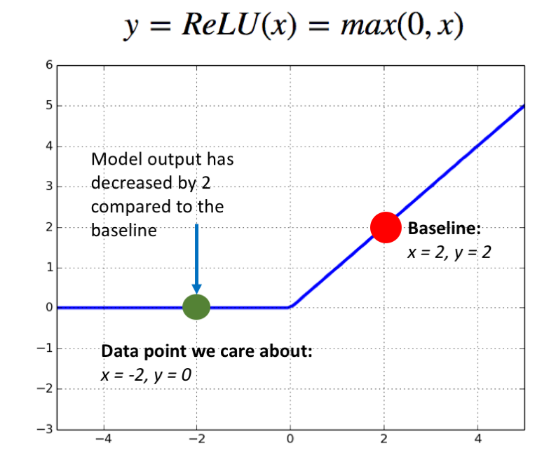
\(ReLU(x=2) = 2 \), and \(ReLU(x=-2) = 0 \), so my input feature \(x = -2 \) has changed the output of my model by 2 compared to the baseline. This change in the output of my model has to be attributed to the change in x, since its the only input feature to this model, but the gradient of \(ReLU(x) \) at the point \(x = -2 \) is 0! This tells me the contribution of x to the output is 0, which is obviously a contradiction.

This happened for two reasons: firstly, we care about a finite difference in the function (the difference between the function when \( x = 2 \) and when \(x = -2 \) ), but gradients calculate infinitesimal differences. Secondly, the ReLU function can get saturated — once x is smaller than 0, it doesn’t matter how much smaller it gets, since the function will only output 0. As we saw above, this results in inconsistent model intepretations, where the output changes with respect to the baseline, but no features are labelled as having caused this change.

These inconsistencies are what Integrated Gradients and DeepLIFT attempt to tackle. They both do this by recognizing that ultimately, what we care about is not the gradient at the point x; we care about how the output changed from the baseline as the input changed from the baseline.

Integrated Gradients

The approach taken by integrated gradients is to ask the following question: what is something I can calculate which is an analogy to the gradient which also acknowledges the presence of a baseline?

Part of the problem is that the gradient (of the output relative to the input) at the baseline is going to be different then the gradient at the output I measure; ideally, I would consider the gradient at both points. This is not enough though: consider a sigmoid function, where my baseline output is close to 0, and my target output is close to 1:

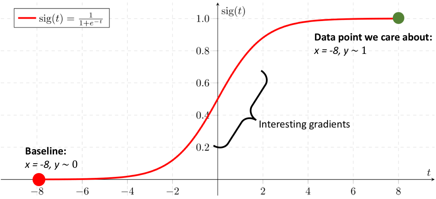
Here, both the gradient at my baseline and at my data point are going to be close to 0. In fact, all the interesting —  and informative — gradients are in between the two data points, so ideally we would find a way to capture all of that information too.

That’s exactly what Integrated Gradients do, by calculating the integral of the gradients between the baseline and the point of interest. Actually calculating the integral of the gradients is intractable, so instead, they are approximated using a Reimann sum: the gradients are taken at lots of small steps between the baseline and the point of interest.

This is extremely simple to implement — in fact, the authors of Integrated Gradients demonstrate a seven-line implementation in their ICML presentation:

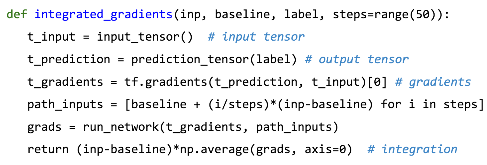
However, the drawback is that since we are approximating an integral, our explanation will also be an approximation. In addition, this method can be extremely time consuming; ideally, we would have small step sizes in our Reimann sum, so that we can closely approximate the integral, but each step requires a backward pass of the network.

DeepLIFT

The approach taken DeepLIFT is conceptually extremely simple, but tricky to implement. DeepLIFT recognizes that what we care about is not the gradient, which describes how y changes as x changes at the point x, but the slope, which describes how y changes as x differs from the baseline.

In fact, if we consider the slope instead of the gradient, then we can redefine the importance of a feature as:

\[ x_{i} \times \frac{\partial Y}{\partial x_{i}} \rightarrow (x_{i} - x_{i}^{baseline}) \times \frac{Y - Y^{baseline}}{x_{i} - x^{baseline}} \]

This is well motivated, since we care about everything relative to the baseline. Applying this to our ReLU network:

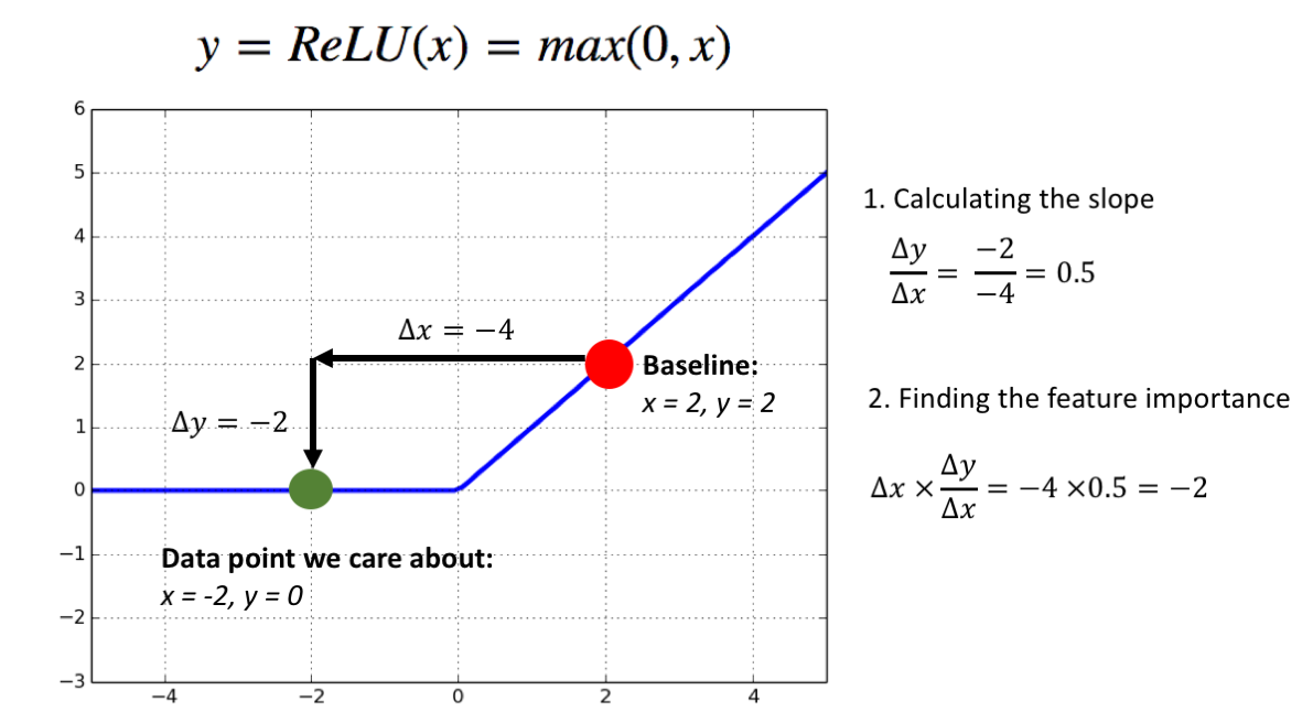
This method tells us that the input x had an importance value of -2. Or, worded another way: “The input x = -2 changed the output of the model by -2 compared to the baseline”. Since this is actually the case, this approach makes a lot of sense.

Now, for each layer, I am going to calculate the slope instead of the gradient, where

\[ \textrm{slope} = \frac{y - y^{baseline}}{x - x^{baseline}} = \frac{\Delta y}{\Delta x} \]

(Note that the inputs and outputs here are of a certain operation — so here, y and x are the outputs and inputs of (for instance) a certain layer in the network.)

DeepLIFT calls this slope a “multiplier”, and represents it symbolically as m. Now that we have redefined the gradient as a multiplier, normal chain rule — and therefore backpropagation — apply, but everything is done relative to the baseline.

\[ \frac{\partial F}{\partial x} = \frac{\partial Y}{\partial x} \frac{\partial F}{\partial Y}\rightarrow \frac{\Delta F}{\Delta x} = \frac{\Delta Y}{\Delta x} \frac{\Delta F}{\Delta Y} \]

Therefore, you can now backpropagate along these multipliers to find the slope of the input with respect to the output of the model, allowing feature importances to be easily defined.

\[ \textrm{feature importance} = (x_{i} - x_{i}^{baseline})\frac{\Delta_{i}Y}{\Delta_{i}x} \]

(Note that I am calculating the ‘partial slope’ of Y, similar to calculating the partial derivative).

The trouble DeepLIFT’s approach to model interpetability is that it redefines how gradients are calculated, meaning you need to dig pretty deep into the guts of most deep learning frameworks to implement it.

The advantage is that it is fast — it only requires one backwards pass of the model to calculate feature importance values — and exact (since, unlike for integrated gradients, there is no approximation that takes place).

Picking a baseline

As promised, we will now return to picking baseline. Aside from some very obvious cases (eg. the MNIST example above), deciding what the baseline inputs are is extremely non trivial, and might require domain expertise.

An alternative to manually picking a baseline is to consider what the prior distribution of a trained model is. This can give us a good idea of what the model is thinking when it has no information at all.

For instance, if I have trained a model on the ImageNet, what is its prior assumption going to be that a new photo it sees if of a meerkat? If 2% of the photos in the ImageNet dataset are of a meerkat, then the model is going to think that the new photo it sees has a 2% chance of being a meerkat. It will then adjust its prediction accordingly when it actually sees the photo. It makes sense to measure the impact of the inputs relative to this prior assumption.

So how can I pick a baseline which is 2% meerkat? Well, a good approach might be to take the mean of the dataset, simply by averaging the images in the dataset together. This is the approach used in the shap library’s implementations of Integrated Gradients and DeepLIFT. Conveniently, it removes the need to be a domain expert to pick an appropriate baseline for the model being interpreted.

Conclusion

Model interpretability continues to be an interesting challenge in machine learning. The biggest problem is that there isn’t a quantitative way to measure one explanation as being better than another; the best we can do is define what properties we would like our explanations to have (such as the sum of the feature importances equalling the difference of the prediction from the baseline).

Hopefully, this post has provided an intuition of two powerful interpretation techniques and how they differ, but there is plenty I haven’t covered (such as what properties the authors of Integrated Gradients and DeepLIFT were optimizing for when they developed their respective techniques), so I encourage taking a look at the papers.

Finally, if you want to experiment with these methods, the shap library has a multi framework implementation of both.

Sources / further reading

Integrated Gradients: Mukund Sundararajan, Ankur Taly, Qiqi Yan, Axiomatic Attribution for Deep Networks, 2017

DeepLIFT: Avanti Shrikumar, Peyton Greenside, Anshul Kundaje, Learning Important Features Through Propagating Activation Differences, 2017

SHAP values: Scott M. Lundberg, Su-In Lee, A Unified Approach to Interpreting Model Predictions, 2017