Montreal Painted by Huang Gongwang: Style Neural Networks

A really cool application of CNNs (convolutional neural networks) recently has been to style neural networks; these involve isolating the style of one image, the content of another, and combining them. For instance, below is an example of style transfer from the first paper to describe it, ‘A Neural Algorithm of Artistic Style’, by Gatys et. al:

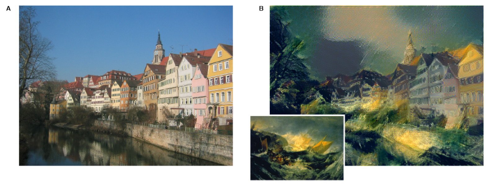
The method of style transfer being used here is based on image iteration. This means that analgorithm will change the image many times (i.e. ‘iterate’) to get an output image.

The main challenge is therefore to describe a loss function which can tell the algorithm whether the image it is creating is closer to or further from what we want.

This is a non trivial problem; how to do you tell an algorithm that you want the shape of the house from image A, but that you want it painted like Joseph Turner’s ‘The Shipwreck of the Minotaur’?

The breakthrough came with the use of convolutional neural networks for image recognition; as a CNN learns to recognize if an image contains a house, it will learn a house’s shape, but its color won’t be important. The outputs of a CNN’s hidden layers can therefore be used to define a Neural Style Network’s loss function.

I’m going to explore Style Neural Networks, and catch up with other developments which have happened with descriptive style transfer based on image iteration since Gatys’ 2014 paper, which first introduced the idea.

The code which accompanies this post can be found here

Contents

Each section in the contents is based on a single paper (linked below each section). My approach to this was basically trying to implement each paper in Keras (and Tensorflow).

1. Getting an intuition for style neural networks, and a basic style neural network (A Neural Network of Artistic Style)

2. Adding more consistent texture throughout the whole image (Incorporating Long Range Consistency in CNN based Texture Generation)

3. Adding Histograms, to remove the variability of Gram Matrices (Stable and Controllable Neural Texture Synthesis and Style Transfer Using Histogram Losses)

4. Combining it all

A basic style neural network

(For basic implementation of a style neural network, I used this post)

Consider how a traditional neural network learns: it will make some conclusion about some data it receives, and then it will adjust its weights depending on if it was right or wrong.

A Style Neural Network works in quite a different way. The weights of the CNN are fixed. Instead, an output image is produced, and the network adjusts the pixels on the image.

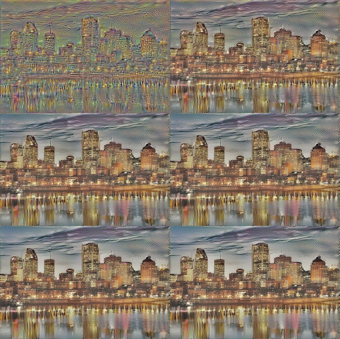
I created the above images using the VGG image recognition model. Style neural networks take advantage of the fact that different layers of the VGG model are good at identifying different things. Later layers are good at identifying shapes and forms (content), while earlier layers recognize patterns and textures (style).

Therefore, if a generated image has a similar output to image A when put through to VGG’s later layers, then it probably has a similar content to image A.

On the other hand, if the generated image has a similar output to image B when put through VGG’s earlier layers, then they probably share a similar style.

With style, there’s an additional twist; calculating the Gramian matrix, and using this as the comparison, instead of the pure output, communicates style far more effectively.

By quantifying the difference between the output of the generated image with the input ‘target’ image (images A and B), I generate a function. This gives me a gradient which I can then use to adjust the pixels of my generated image (using gradient descent).

I can quantify the difference as the mean squared error between the VGG model’s outputs for both the generated and target images:

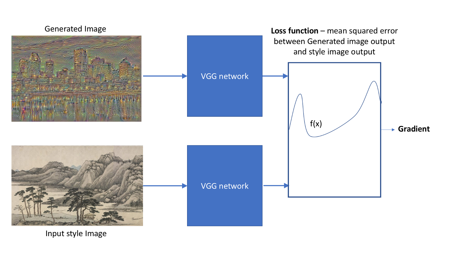
The above image describes creating a loss function. The loss function, and gradient, are recalculated at every iteration. The gradient is a matrix of the same size as the generated image (with two additional dimensions, for the RGB channels), so that each pixel is changed according to the gradient value for that pixel.

Note: from now onwards, when I say I am comparing images (eg. comparing the generated image to the style image), what I mean is that I am comparing the VGG output.

What does the content and style side of the neural network actually aim for? I can visualize this by starting from random noise, and only using the content or loss function to see what image each side of the neural network is trying to generate:

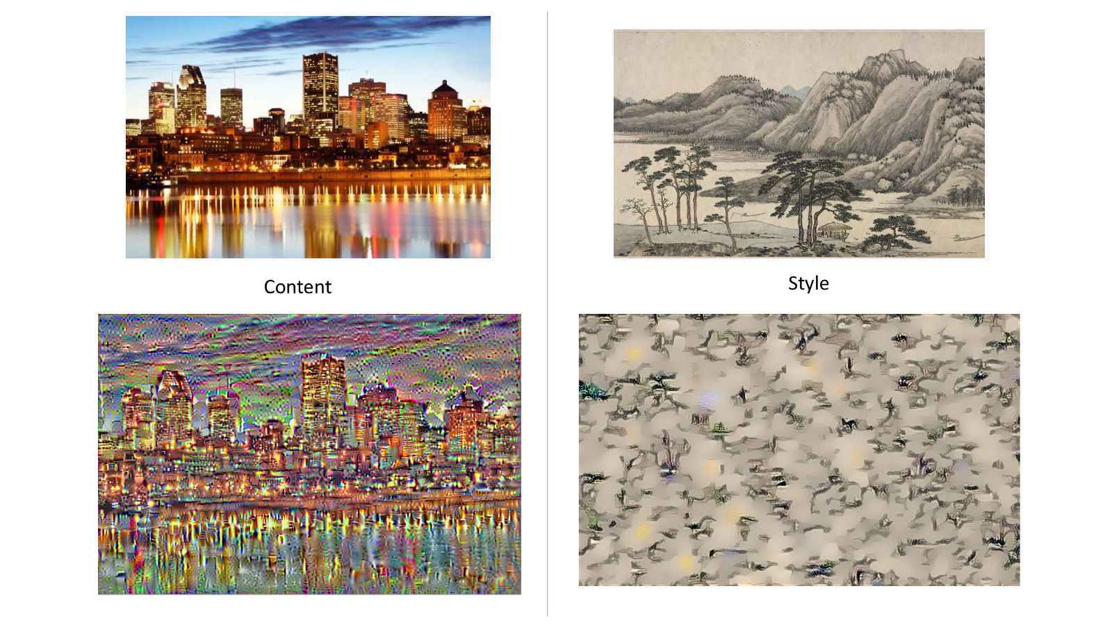
Starting from random noise, only using the content loss function with the Montreal skyline as content input yields the bottom left image. Only using the style loss function with the Fuchun mountains as style input yields the image on the bottom right. In both cases, the network was run for 10 iterations.

Then, combining the style and loss functions together yields:

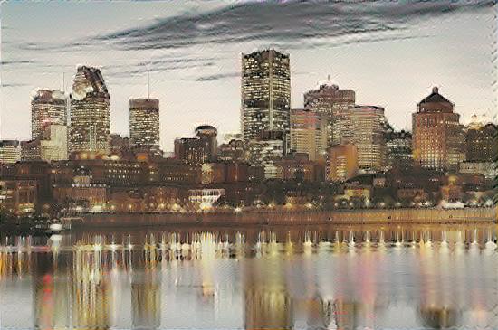
Note: as per Novak and Nikulin’s recommendations, I used the content image as the starting image, instead of random noise.

This is a super cool start to combining images, but has a few shortcomings. Luckily, there’s been lots of work by later researchers to tackle them. I’m now going to try implementing some of these solutions to get a nice image of Montreal, as painted by Huang Gongwang.

Incorporating Long Ranged Consistency

The gram matrix of X is the dot product of itself to its transpose: \( X \cdot X^{T}\). This compares each element of X to itself, and is good at getting a global understanding of what is going on in the image.

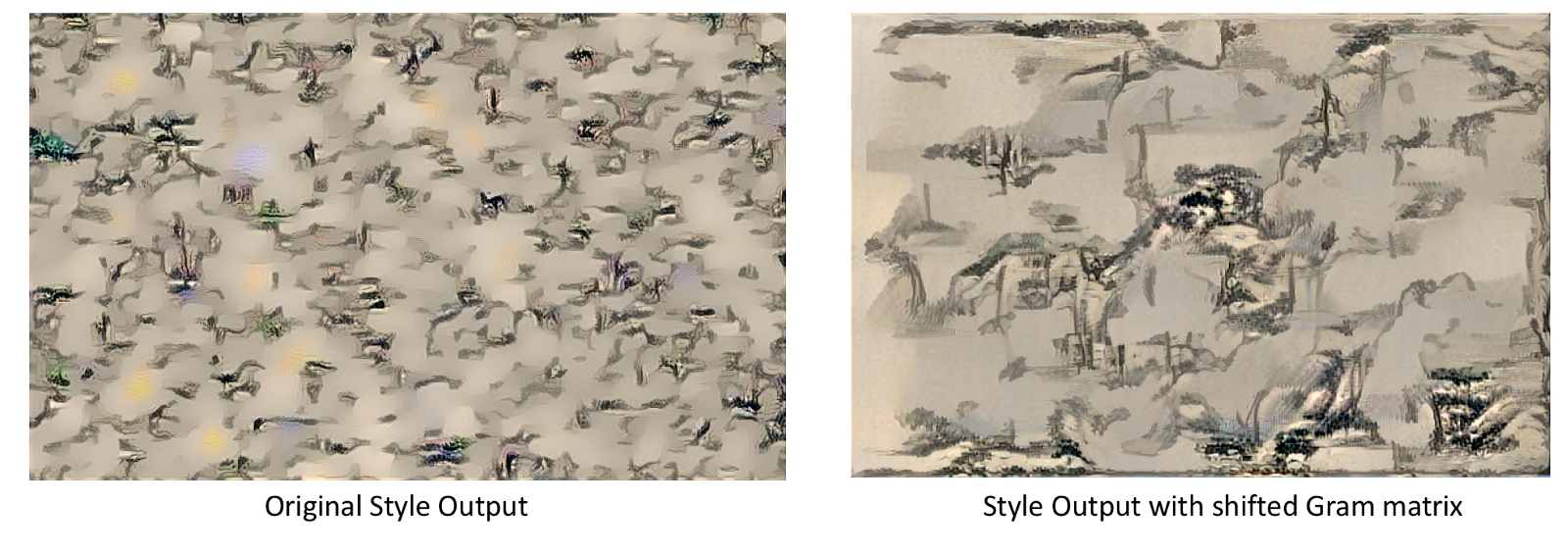
However, this fails to capture local structure within an image. A way to compare local structure would be to compare each element not just to itself, but to its neighbours as well. There’s an easy way to implement this; just translate the outputs sideways a little when calculating the gram matrices: (credit to the original paper for this figure)

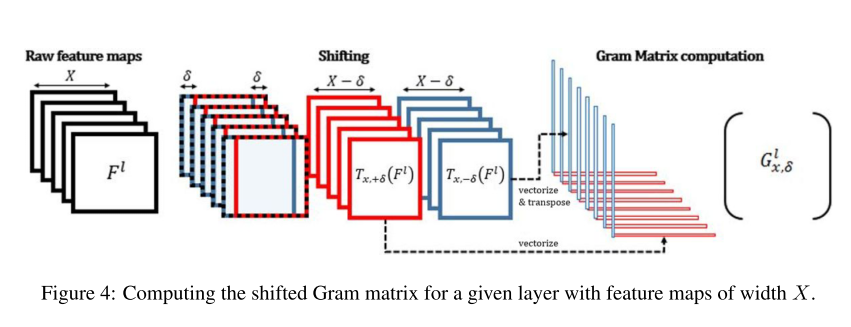
Implementing this slight change to the style loss function has a significant effect on the output:

Histogram Loss

There’s a big problem with using Gramian matrices to measure the style, and this is that different images can yield the same Gram matrix. My neural network could therefore end up aiming for a different style than what I want, which coincidentally generates the same Gram matrix.

This is a problem.

Luckily, there is a solution: histogram matching. This is a technique which is currently used in image manipulation; I take a histogram of the pixel colours in a source image, and match them to a template image. For instance, in ali_m’s image below, grayscale histogram matching is applied to two images:

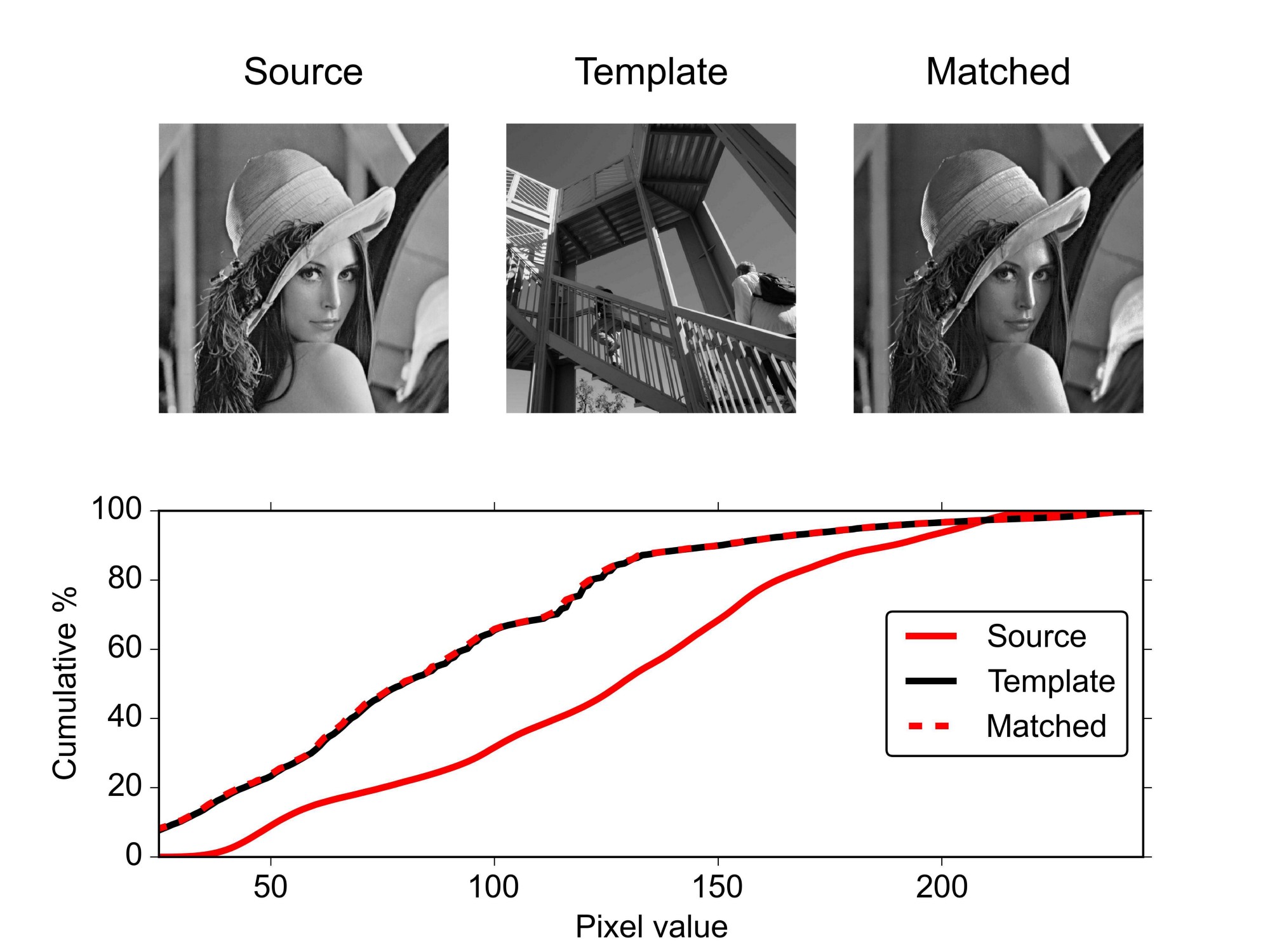
The same principle can be applied to my image outputs. By using my generated image as the source image, and the target style image as the template image, I could then define my loss as the difference between the generated image and the target style image.

In the image below, I apply histogram matching with the target outputs. The jitteriness of the matched histogram can be attributed to the number of histogram bins; I plotted this using 255 bins. Using every unique output layer value as a bin would have been desirable, but computationally impossible (there were about 5 million unique values). This jitteriness was therefore the tradeoff for reasonable computation times.

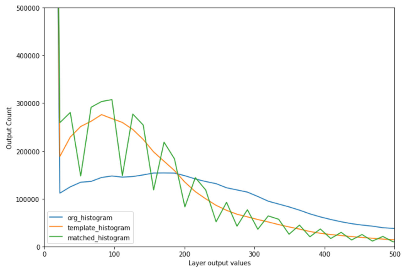
Now, given my generated image and my matched image, I can define my loss as the mean squared error between the two. This new histogram loss can then be added the loss generated by the Gramian matrix, to stabilize it.

Combining it all, with additional improvements

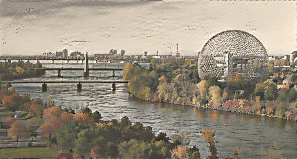
Combining these two losses to the original content and style losses, I then used as a style image Dwelling in the Fuchun Mountains and as input, this image of Montreal’s biosphere.

Takeaways

1. Leave the network alone! When generating the last image, I had a tendency to ‘micromanage’ my network, and change the parameters as soon as the loss stopped decreasing. Just letting the network run yielded the best results, as it tended to get out of those ruts.

2. Its especially hard to tune the parameters for Style Neural Networks, because its ultimately a subjective judgement whether or not one image looks better than the next. Also, some images will do a lot better than others.

3. Tensorflow is tricky. In particular, evaluating a tensor is the only way to make sure everything is working; tensorflow may say an operation is fine, and only throw up an error when its being evaluated.